Experience Replay in Machines and Mammals

Experience replay is a fascinating topic spanning machine learning, neuroscience and cognitive science. At the heart of replay are 3 questions, asking how an agent should use its past experiences:

1. to build a model of its world
2. to most efficiently propagate reward information in that model
3. to plan future actions using that model

The machine learning literature has historically focused on the second question, but emerging work in neuroscience and cognitive science suggests that these three questions are intimately related. This story begins with the second question and continues to the forefront of the third and first questions.

Papers covered:

• Minh et al. 2015 Human-level control through deep reinforcement learning
• Schaul et al. 2016 Prioritized experience replay
• Mattar and Daw 2018 Prioritized memory access explains planning and hippocampal replay
• Liu et al. 2021 Experience replay is associated with efficient nonlocal learning
• A few others briefly

Notation

In reinforcement learning (RL), one common mathematical framework is to consider an agent in a Markov Decision Process (MDP). An experience is often defined as a 4-tuple of an agent’s state, the action it takes, the reward it receives and the next state it ends up in:

\[e_k = (s_k, a_k, r_k, s_{k+1})\]

As an agent moves through its environment, it builds a collection of these experience \(E_T := \{e_1, ..., e_T\}\) called a “replay buffer”.

Lin 1992 & Minh et al. 2015

In the early days of RL, a hot topic was model-free value-based RL: Q learning. The original approach to Q-Learning was when an agent obtains a new experience, it should use that experience to immediately perform a Bellman backup:

\[Q(s_t, a_t) \leftarrow Q(s_t, a_t) + \eta_t (r_t + \gamma \max_a Q(s_{t+1}, a) - Q(s_t, a_t))\]

where \(\eta_T\) is some learning rate. The experience is then discarded. In 1992, Lin suggested the idea of experience replay, that instead of discarding past experiences immediately, the agent should store those experiences in its replay buffer and then uniformly sample from the buffer. Two decades later, experience replay proved critical in Minh et al.’s 2015 DQN Nature paper that kickstarted the field of deep reinforcement learning:

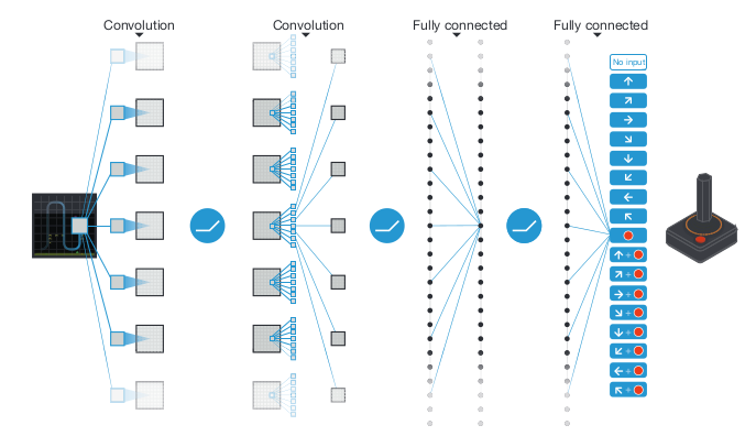
Many people remember the paper for showing that deep Q-Learning can surpass human performance at Atari games, but the authors were clear that experience replay was no less important:

"Notably, the successful integration of reinforcement learning with deep network architectures was critically dependent on our incorporation of a replay algorithm involving the storage and representation of recently experienced transitions."

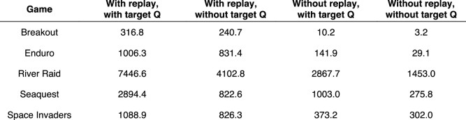
The specific replay mechanism was a queue (FIFO) with a capacity of 1 million experiences. that sampled experiences uniformly at random, on average 8 times. Note that because Q-learning is model free, these experiences were not used to learn a model of any environment. On the 5 games the authors used for prototyping, removing replay eviscerated the agent’s performance.

Schaul et al. 2016

At ICLR 2016, Schaul et al. proposed that sampling experiences uniformly at random might be a suboptimal approach. They suggested that the agent could instead prioritize certain experiences, using the heuristic of how wrong the agent’s predictions were. Specifically, Schaul et al. suggested that when sampling experiences, the agent should take into account its temporal-difference (TD) errors \(\delta_t\) (also known as reward prediction errors):

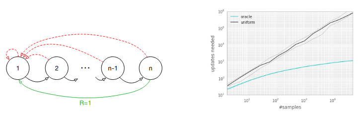
\[\delta_t := R_t + \gamma \max_a Q(S_{t+1}, a) - Q(S_{t}, A_{t})\]

As a motivating example, the authors present the “Blind Cliffwalk” environment, in which there is a sequence of \(n\) states, each state has 2 actions and in order to reach the goal state, the agent must choose the correct action in each state or else go back to the beginning. If the agent samples uniformly over its experiences, it needs a massive number of samples and updates to learn to reliably reach the goal, whereas an oracle (which greedily selects a transition that maximimally reduces the global loss) requires significantly fewer samples and updates.

However, the agent can’t just greedily select the experience with the highest TD error, for at least 2 reasons:

1. The agent will overfit to experiences with high TD errors because states with low TD error will never be replayed
2. If rewards are stochastic, high TD errors will be monopolized by tails of the reward distributions

Instead of greedily selecting experiences to replay, Schaul and colleagues propose that experiences should be sampled randomly. They propose two different ways to define the priority of the \(k\)th experience

1. Direct: \(p_k := \lvert \delta_k \lvert + \epsilon\), where \(\epsilon > 0\) is a small positive constant to ensure even experiences with no TD error have a chance at being replayed
2. Indirect: \(p_k := \frac{1}{rank(k)}\), where the rank is determined by the ordered TD errors

and then sample experiences proportional to the priority:

\[p(e_k) = \frac{p_k^{\alpha}}{\sum_{k'} p_{k'}^{\alpha}}\]

They then introduce one other change: they use importance sampling weights, defined as:

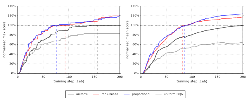
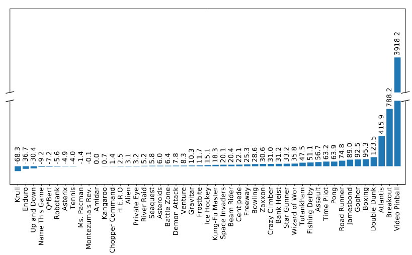
\[w_k := \Big( \frac{1}{N p(e_k)} \Big)^{\beta}\]

They found that both prioritization approaches yielded similar boosts in max and average performance on the Atari suite of games

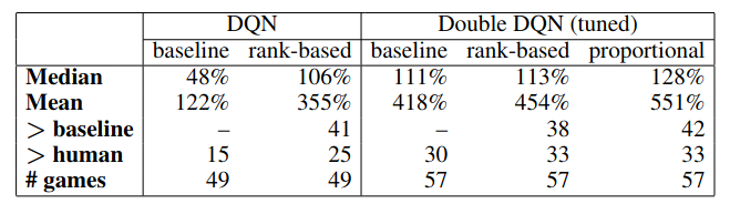
They also found that learning was faster for the prioritized replay agents.

As a disclaimer, the authors later write “Note that mean performance is not a very reliable metric because a single game (Video Pinball) has a dominant contribution.” If that’s the case, I don’t understand why max score is a more reliable metric, since surely the same problem exists there?

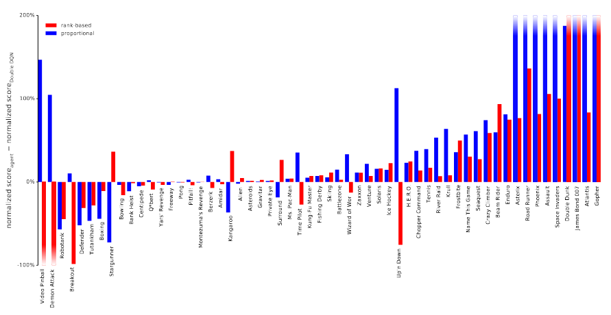
Looking at each game individually, they found that while the effect of the replay sampling differed depending on the game, both replay mechanisms typically offered an improvement.

Prioritized Experience Replay: Questions and Details

Questions

• Why did they only try their sampling on Double DQN and not DQN? What impact does prioritize replay have on DQN?
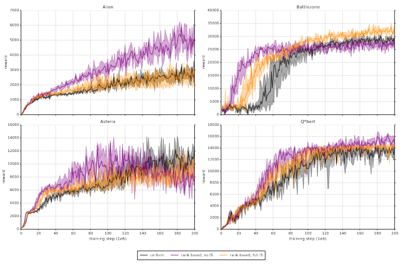
• The paper claims that the importance sampling (IS) weights are useful and offers a handwavy explanation for why. Are there any ablations testing the effects of not using the IS weights?
  • Fig 12 in the appendix contains such ablation tests, but only for 4 environments and only for rank-based sampling. Honestly, this evidence seems to suggest not only that IS is not critical but that uniform is indistinguishable from rank-based no IS and from rank-based IS.

Other heuristics

After the Prioritized Experience Replay paper came out, other groups started exploring their own heuristics for choosing how to prioritize experiences.

Episodic Backward Update

In 2019, Lee, Sungik and Chung proposed “Episodic Backward Updates” (EBU), which uniformly samples an episode from the replay buffer, then replays state-action pairs in reverse order. The authors claim that agents trained using EBU are significantly more sample efficient, although the comparisons are spotty (in fairness, training RL agents to play every Atari game is really compute intensive). Here they compare their replay mechanism against the uniform replay sampling used by Minh et al. 2015.

Topological Replay Experience

For instance, in 2021, Hong, Chen, Lin, Pajarinen and Agrawal proposed “Topological Experience Replay” (TER) which, after a high rewarding state has been reached, propagates backward in the graph of state-state transitions so that the states which lead to the rewarding state can have their action values updated:

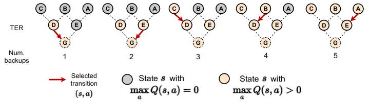
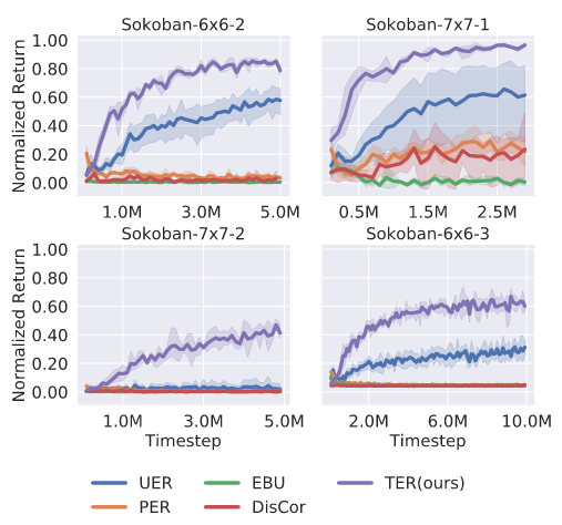
More specifically, if the agent has the transition function \(T: S \times A \rightarrow S\) or an accurate approximation of the transition function, the agent can construct the graph of state-state transitions. Then, the agent performs breadth-first search, starting from each terminal vertex and moving backward. They also interleave Prioritized Experience Replay backups because they found this works better empirically (their experiments don’t disentangle what effect PER had). On Sokoban, the block pushing game, they learn significantly faster than other replay methods:

Mattar and Daw 2018

In 2018, Mattar and Daw presented a beautiful and simple idea. Rather than proposing a heuristic for prioritizing experience, they asked: could the problem of choosing experiences be written as an optimization problem? The answer was yes! For a deeper dive, read my blog post, but I’ve included a high level summary here.

Mattar and Daw’s approach starts with consider what effect replaying an experience will have. Suppose the agent is in state \(s_t\) and considers replaying experience \(e_k\). Before replaying that experience, the agent has some value function for its current state:

\[V^{\pi_{old}}(S = s_t) := \mathbb{E}_{\pi_{old}} \Big[ \sum_{i=t}^{\infty} \gamma^i R_{i+1} \Big]\]

After replaying that experience, the agent has a new (although possibly identical) value function for its current state:

\[V^{\pi_{new, k}}(S = s_t) := \mathbb{E}_{\pi_{new, k}} \Big[ \sum_{i=t}^{\infty} \gamma^i R_{i+1} \Big]\]

Mattar and Daw’s idea is that the agent should choose to replay whichever experience maximizes the increase from the old value function in the current state to the new value function in the current state i.e. how much more value the agent will accrue moving forward. They pose the following optimization problem:

\[\arg \max_{e_k} V^{\pi_{new, k}}(S = s_t) - V^{\pi_{old}}(S = s_t)\]

They term this improvement, this difference, the Expected Value of Backup:

\[EVB(s_t, e_k) := V^{\pi_{new, k}}(S = s_t) - V^{\pi_{old}}(S = s_t)\]

Mattar and Daw then show that the expected value of a backup can be decomposed into the product of two terms:

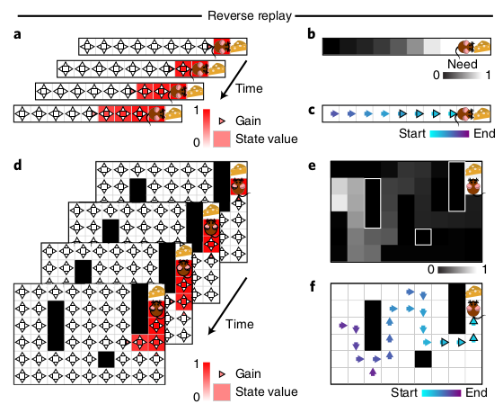
1. Need: How likely is the agent is to find itself in \(s_k\) in the future?
2. Gain: How much more value will the agent accrue in \(s_k\), following \(\pi_{new, k}\) instead of \(\pi_{old}\)?

The need and gain are defined as:

\[\begin{align*} EVB(s_t, e_k) &:= Need(s_t, s_k) \, \, Gain(s_k)\\ Need(s_t, s_k) &:= \sum_{t' = t}^{\infty} \gamma^{t' - t} \delta(S_{t'}, s_k)\\ Gain(s_k) &:= \sum_{a \in A} Q^{\pi_{new, k}} (s_k, a) \Big(\pi_{new, k}(a|s_k) - \pi_{old}(a|s) \Big) \end{align*}\]

In their simulations, Mattar and Daw assumes that the agent solves this optimization problem by brute force i.e. computing each experience’s EVB and then replaying the experience with the highest EVB. Before showing the wealth of experimental phenomena that this approach can explain, we should acknowledge some of its shortcomings:

• This approach only works for a known, discrete state space and a known transition function \(P(s_{t+1} \lvert s_t, a_t)\)
• The proof assumes that changing the agent’s policy in one state has no effect on the agent’s policy any other state. This is unrealistic if the agent uses function approximation.
• The proposed prioritization scheme is circular, in that when deciding whether to replay an experience that will change its action value function, the agent must first compute the action value function after replaying the experience \(Q^{\pi_{new}}\), which requires performing the backup!
• The optimization problem is greedy, in that it asks for the single best experience to replay
• Their solution to the optimization problem is to compute the EVB for each experience and is therefore linear in the number of experiences at each time step
• The theory doesn’t explain when to replay, just what to replay (although see Agrawal, Mattar, Daw and Cohen 2020)

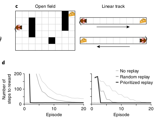
Mattar and Daw consider two abstract versions of tasks used by mouse experimentalists: the open field and the linear track. They show that their prioritized replay learns to significantly faster learning:

Two experimental phenomena that Mattar and Daw are interested in are (a) reverse replay and (b) reverse replay. Reverse replay refers to when a sequence of hippocampal cells fire starting from the animal and typically tracing the animal’s path backwards, whereas forward replay refers to when a sequence of hippocampal cells fire starting from the animal’s current position and tracing the path the animal will take. Reverse replay almost always occur at the end of a trial and forward replay almost always occurs at the start of a trial:

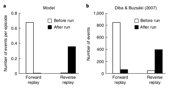
In Mattar and Daw’s model, reverse replay occurs when the animal encounters a reward, it now wants to propagate that reward information backwards (i.e. gain dominates) to know how to return to the reward location.

In contrast, forward replay occurs when the animal needs to figure out where to go. Despite its name, forward replay produces mental trajectories that look like planning.

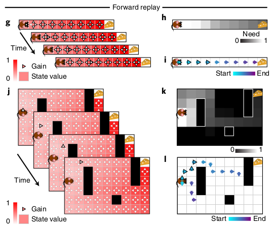
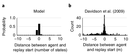
In the model, replay almost always starts from the animal’s current position, matching experimental data.

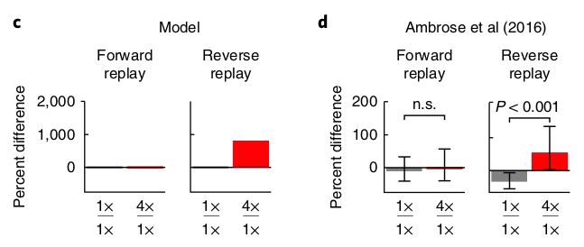
Next, Mattar and Daw explain asymmetric effects of positive and negative prediction errors. Ambrose et al. tried increasing the reward four-fold in half the trials and found that forward replay was unaffected but reverse replay increased. This is caused by more reverse replay for 4x reward trials and fewer reverse replay for 1x reward trials.

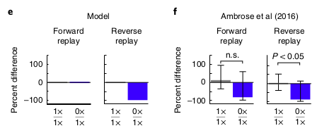
However, when the authors tried decreasing the reward to 0 in half the trials, they again found no effect on forward replay, but that no reward has a negative effect on reverse replay, which is caused by more reverse replay for 1x trials and less replay for 0x trials.

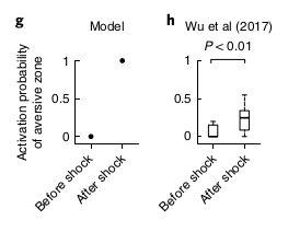
However, Wu and colleagues found a difference result if the reward is negative (i.e. a shock) instead of just zero: the amount of reverse replay increases. The model explains this because a negative reward prediction error only matters if a better option is available; since the mice are running back and forth on a linear track, 1 reward or 0 reward is better than not running, but when the shock is introduced, 0 reward or -1 reward means that the animal should stop running.

As a side note, Daw mentioned in a talk that if we assume that place cell trajectories are performing model-based simulation, we can learn that:

• Simulation can occur forward (planning), backward (learning) and nonlocally
• Simulation only occurs when animal is stopped
• Simulation occurs one path at a time

Daw thinks these last two are probably because hippocampus is an attractor network and can only represent 1 path at a time. He thinks that the path field neural code can track the animal’s current location or an imagined location, but not both simultaneously.

Liu, Mattar, Behrens, Daw and Dolan 2021

Mattar and Daw wanted to test their theory of how agents prioritize experiences to replay, and so turned to collaborate with Liu, Behrens and Dolan. They sought to test two hypotheses:

1. Does trajectory replay support non-local learning?
   • Do people learn more about replay paths?
2. Are learning and replay prioritized?
   • Behaviorally, do people learn more about high (need * gain) paths?
   • Neurally, do people preferentially replay high (need * gain) paths?

To explain the bit about non-local learning, we need to take a step back. Daw believes that RL is hard because it requires connecting actions to consequences non-locally, often called “temporal credit assignment.” The point about non-local learning is that information about one location of a task may be important for a distant part of the task, and replay needs to connect these two components to support efficient learning.

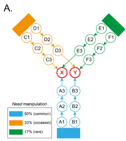
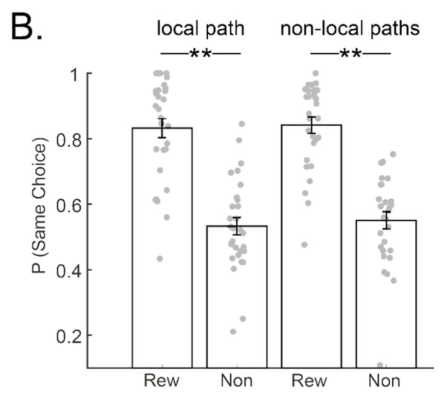
Liu and the team put humans in the following task: there were three start states (orange, green and blue), and 2 paths from each start state; each path ended in one of two possible end states, with different (drifting) probabilities of receiving a reward. Along each path, humans were shown a sequence of natural pictures (e.g. a zebra at A1, a soccer ball at A2, etc.).

Non-locality is important here because some paths tell the participant about other paths. For instance, suppose I take path A and receive a high reward; if I understand the structure of the task, and I start the next trial on Green, I should take path E because I know X is highly rewarded. Liu et all found that behaviorally, if humans were placed back in the same start state (e.g. blue, followed by blue), humans were more likely to take the same path on the second trial if they received a reward on the first trial; more interesting, humans were more likely to take an equivalent path on the second trial if rewarded on the first, providing behavioral evidence of non-local learning.

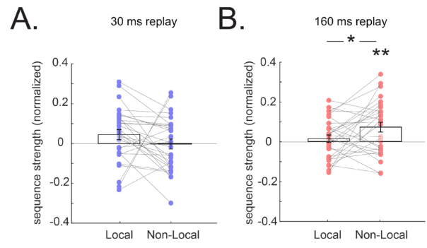
Using MEG, Liu et al. found two replay events: forward replay around ~30 ms and slow replay around ~160 ms.

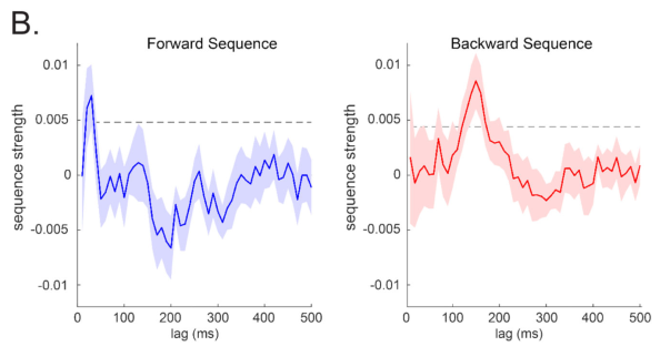
The forwards replay showed no preference for the local path, but the backwards replay showed a preference for non-local learning:

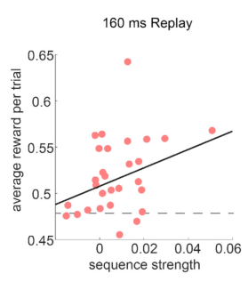
There was a strong correlation between 160 ms lag replay and task performance across subjects.

Finally, the authors confirmed their hypothesis that the model which best explains the backwards replay at 160 ms was not need, not gain, but the product of need times gain (p = 0.003). Weirdly, the forward replay showed no preference for any of the three.

Theory

https://ieeexplore.ieee.org/abstract/document/8636075

Empirical Study

http://proceedings.mlr.press/v119/fedus20a.html

https://arxiv.org/pdf/1712.01275.pdf

Replay for Changing Goals

https://arxiv.org/abs/1707.01495

https://arxiv.org/pdf/1906.08387.pdf

Replay in Continual Learning

https://arxiv.org/abs/1811.11682

https://ojs.aaai.org/index.php/AAAI/article/view/11595